Calculating Extinction
Background
Extinction is generally measured by comparing two stars that are identical in their physical properties, differing only in that one is seen through more dust than the other. Finding two stars with identical properties is straightforward as it just means finding two stars with the same 2D spectral types (temperature and luminosity) and the same metallicities. As a result, measuring extinction is a simple matter of dividing the observations of the two stars and a small amount of math to convert this to magnitudes. Using observations taken with the same instrumentation for both the reddened and comparison star means that only good relative calibration is needed. Instead of using observations of a star with little to no reddening, a model stellar atmosphere can also be used (e.g., Fitzpatrick & Massa 2005). This can provide a better match, but it comes at the expense of requiring good absolute calibration.
The basic measurement is giving the magnitude excess relative to a reference wavelength measurement. The reason for using a reference wavelength is that the distance to a star is rarely known to high enough accuracy to directly measure the extinction at a single wavelength. Thus, the basic measurement gives the relative extinction between two wavelengths. Usually, the V band measurement is used as the reference. Thus, the dust extinction at wavelength \(\lambda\) is:
where \(m(\lambda - V)\) is the difference in magnitudes between the flux at \(\lambda\) and in the V band, \(m(\lambda)\) is the magnitude, \(F(\lambda)\) is the flux, \(r\) refers to the reddened star, and \(c\) refers to the comparison star. Note that since \(E(\lambda - V)\) is a differential measurement there is no dependence on the zero point of the magnitude system.
This extinction measurement can be normalized allowing comparison with extinction along other lines-of-sight. The normalization is often done to \(E(B-V)\) as this is easily measured. But notice that this is a normalization to a differential measurement.
Converting the \(E(\lambda-V)\) differential measurement to the \(A(\lambda)\) absolute measurement requires knowledge of the absolute extinction at the reference wavelength, V band in this case. Determining \(A(V)\) requires measuring \(E(\lambda-V)\) at the longest wavelength possible and extrapolating with a reference shape to infinite wavelength as \(A(inf) = 0\). Usually, the longest wavelength measured is the K band and the extrapolation to infinite wavelength is on the order of 10% (Whittet, van Breda, & Glass 1976; Fitzpatrick & Massa 2009). With a measurement of \(A(V)\) then an absolute normalized extinction measurement is possible using
With a measurement of \(E(B-V)\) and the extrapolated measurement of \(A(V)\), then the total-to-selective extinction can be computed as this is \(R(V) = A(V)/E(B-V)\). \(R(V)\) is diagnostic of the average behavior of dust extinction as a function of wavelength (Cardelli, Clayton, & Mathis 1989; Valencic et al. 2004; Fitzpatrick & Massa 2007; Gordon et al. 2009). The \(R(V)\) dependent relationship for the average extinction behavior does not give the full picture as extinction curves in the Magellanic Clouds strongly deviate from this relationship (Gordon et al. 2003).
Terminology Summary
\(m(\lambda - V)\) = magnitude difference between \(\lambda\) wavelength and V band
\(m(\lambda)\) = magnitude at \(\lambda\)
\(F(\lambda)\) = flux at \(\lambda\)
\(E(\lambda - V)\) = extinction excess between \(\lambda\) wavelength and V band
\(A(V)\) = V band extinction
\(R(V) = A(V)/E(B-V)\) = total-to-selective extinction
Example
Spectra
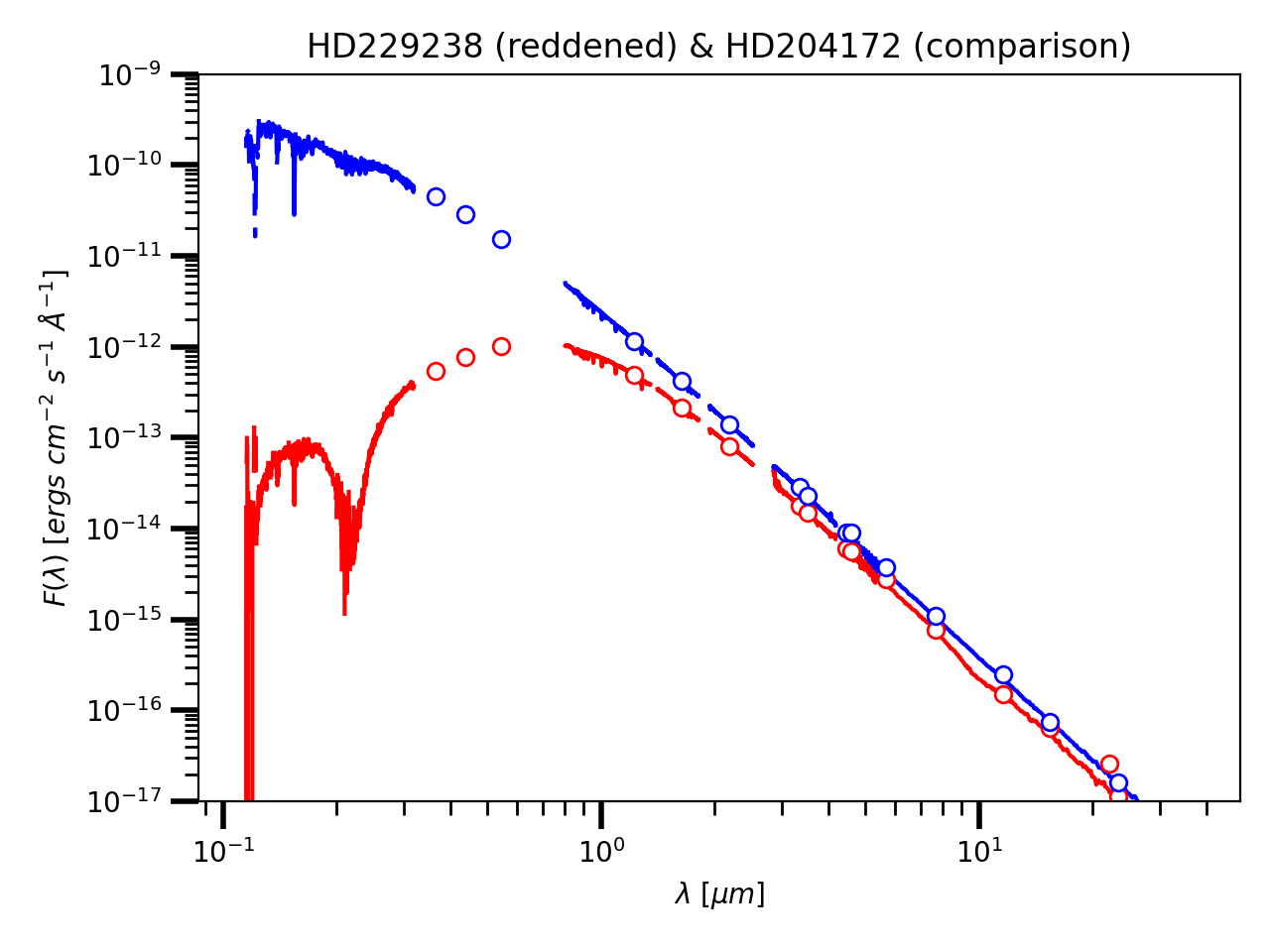
HD229238 and HD204172 are two stars with similar spectral types that have observed UV spectra from IUE, NIR spectra from SpeX, MIR spectra from IRS, optical and NIR photometry from ground-based observations, and NIR/MIR photometry from IRAC, WISE and MIPS. These two stars differ in that HD229238 is seen through a large column of dust and HD204172 is seen through very little.
The data files (.dat) for both stars are given in the data directory for this
package along with the observed spectra (in Spectra).
For details of the format of these files, see Data Formats.
Using these files, the spectra of both stars can be plotted by reading in the
observed data using the StarData object
and then calling its member function plot.
import matplotlib.pyplot as plt

from measure_extinction.stardata import StarData
starobs = StarData(dat_filename)

fig, ax = plt.subplots()
starobs.plot(ax)
The spectra for both stars are plotted using those data files. Which star is reddened is clear as it has a non-stellar slope for an early type star and clearly shows the 2175 A absorption feature.
(Source code, png, hires.png, pdf)

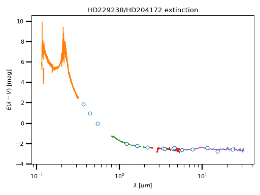
Extinction
Measuring the extinction is done by reading in observed data for both
stars into StarData objects and
then using an ExtData object and its
calc_elx member function. The calc_elx function ratios the reddened to
the comparison star relative to any band (x) and coverts the results to magnitudes
resulting in \(E(\lambda - x)\). The plot can then be shown using the
member function plot_ext.
import matplotlib.pyplot as plt

from measure_extinction.stardata import StarData
from measure_extinction.extdata import ExtData

redstar = StarData(red_dat_filename)
compstar = StarData(comp_dat_filename)

extdata = ExtData()
extdata.calc_elx(redstar, compstar)

fig, ax = plt.subplots()
extdata.plot(ax)
(Source code, png, hires.png, pdf)
Normalization
One common normalization is to divide by \(E(B-V)\). As long as
both the data used for the reddened and comparison stars include B and V
measurements, \(E(B-V)\) has already been calculated. The
ExtData member function trans_elv_elvebv
performs this normalization while checking that the B band measurement
exists.
extdata.trans_elv_elvebv()
(Source code, png, hires.png, pdf)

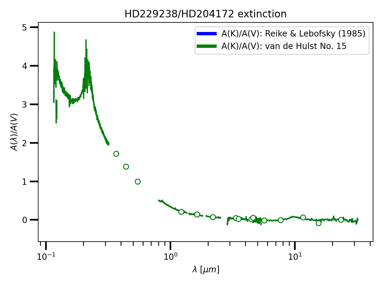
Another common normalization is by \(A(V)\). This provides an absolute normalization instead of the differential normalization provided by \(E(B-V)\). In order to determine \(A(V)\), the \(E(\lambda-V)\) curve is extrapolated to infinite wavelength as \(A(inf) = 0\), thus \(E(inf - V) = -A(V)\). In general, the longest wavelength easy to measure is K band so \(E(K - V)\) is often the measurement to be extrapolated. To do this extrapolation, a functional form of the extinction curve at the longest wavelengths must be assumed. One choice is to assume the near-/mid-IR extinction curve from Rieke & Lebofsky 1985. The value for the K band extinction is given in Table 3 of this reference as \(A(K)/A(V) = 0.112\).
The ExtData member function trans_elv_alav
performs this normalization.
(Source code, png, hires.png, pdf)
Other choices for \(A(K)/A(V)\) can be used by setting the parameter akav in this member function.
# value from Rieke & Lebofsky (1985)
extdata.trans_elv_alav(akav=0.112)

# use value for van de Hulst No. 15 curve instead
extdata.trans_elv_alav(akav=0.0885)
Comparison to Models
Compute R(V).
Show comparisons to existing R(V) dependent models using dust_extinction.